AmateurRadio.com

International Ham Radio News & Opinion

Posts Tagged ‘Digital mode’

All continents in one night on WSPR

April 2nd, 2015 |

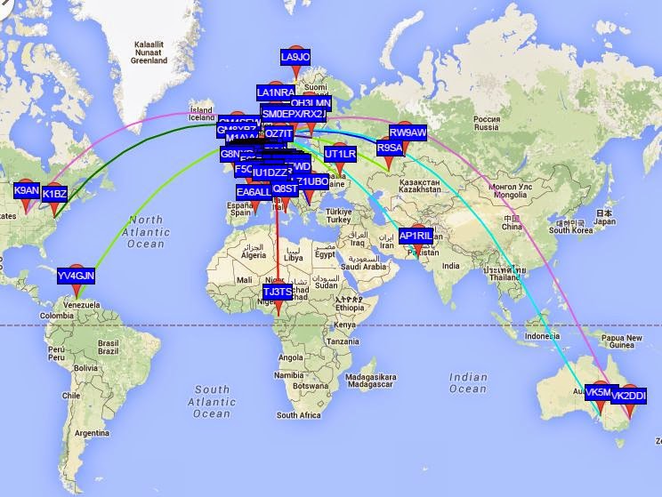
For me South America, Australia, and Africa are quite rare on WSPR. But they all heard my tiny 0.2 W signal the night between 31 March and 1 April in addition to North America, Asia and Europe. That’s a new one for me and worthy a brag post on the blog, I think! Hopefully, it may also inspire others to try low power WSPR.

In Australia and South America I was heard on the 10 MHz band, in Africa on 21 MHz, in Pakistan on 14 MHz, while 7 and 10 MHz worked into Siberia. North American stations also heard me on the 7 and 10 MHz bands.

This was on my untuned 80 m horizontal loop fed with open-wire feeder and a 4:1 balun. This shows both that the bare-foot Ultimate 3 kit is very tolerant of loads with SWR much different from 1, and that WSPR gives amazing results.

WSPR on 5 bands

August 7th, 2014 |

Author: Sverre LA3ZA

For the first time ever I have been spotted on all the five bands that my Ultimate3 QRSS/WSPR kit (G0UPL design) is transmitting on. This is after 2-3 days of transmitting.

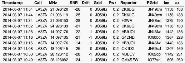
Right now I am using the beacon for discovering if the bands should open up on 24 and 28 MHz. The other three bands, and especially the 14 MHz band, serve as references to tell me that the transmitter is working. My antenna is not so optimal so I would be surprised if I am spotted far outside Europe. It is an end-fed 5 m long half wave vertical dipole which isn’t too bad for 28 and 25 MHz, and probably not very good at all on 21, 18, and 14 MHz.

Ultimate QRSS kits

February 3rd, 2014 |

Author: Sverre LA3ZA

I’m a great fan of Hans Summers (G0UPL) and his effort in launching kits for various slow speed modes. In fact I have all three generations of the Ultimate QRSS kits up and running. That includes the original single-band kit (30 m in my case, bottom in picture), as well as number 2 and 3, the multi-band kits.

The latest version, in the middle of the picture, has a nicer two line display, and it can also be fitted with a relay board. It makes it possible to jump between up to 6 different bands.

I have used them exclusively in the WSPR mode so far. For time synchronization with the first and last version I have used an EM-406 GPS module which also provides the required pulse-per-second output. My Ultimate 2 has a too early software revision to work with the GPS, so it is on my list for a firmware upgrade.

I have a lot more experimentation to do before I know these kits and their capabilities, but I have at least gotten some experience with how far 150 mW of WSPR can take you, and that was to Australia on 30 m in my case. This is really amazing.

I would recommend the latest kit to anyone who is interested in experimentation with digital modes and who wants to compare e.g. antennas or just observe how propagation varies. The price is reasonable also, starting at GBP £17.50.

The challenge for me has been to find suitable enclosures for the two last kits. I hope to be able to make something from plexiglass for the last one. But I am still looking for that great idea for how to do that.

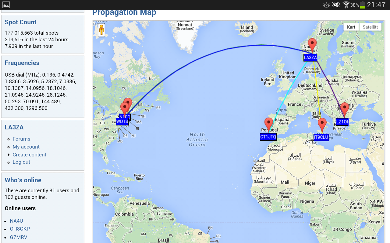
The last 24 hours on 10 m with a horizontal loop antenna, 80 m long, has caused my tiny signal to be decoded in the US several times as shown below.

See also “My first 24 hours on WSPR” and the G0UPL pages.

Elecraft K3 modifications

October 29th, 2013 |

Author: Sverre LA3ZA

There aren’t that many modifications that you can do to the Elecraft K3. This is very different from the K2 as in my list I now have 138 different modifications for it. But Elecraft does have a few K3 enhancements and mods on their home page and here are two additional modifications that I have done to my K3.

Plug-in roofing filters on
main RX board

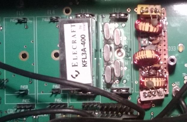
The first one is to add a wideband LC-filter (roofing filter). The filter was inspired by ideas from W5DHM with three tuned sections at the IF frequency of 8.215 kHz. It is to the right in the image. It is not the best of filters, and probably compromises performance somewhat, most likely because of its low image rejection 30 kHz away. It has however served me well as a receiver filter for the latest version of K1JT’s software WSJT-X. That software processes a 4 kHz band for both the JT65 and JT9 digital modes, and the LC-filter has demonstrated to me the utility of having a wide roofing filter for reception of those modes. The filter also works well for listening to broadcast AM which was what W5DHM designed it for in the first place.

Back panel of the K3

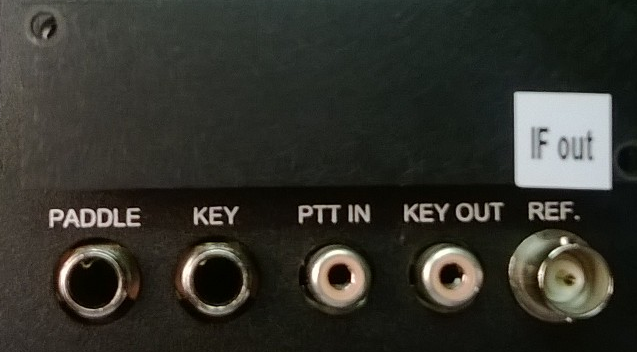
The second modification allows for a connection to the P3 Panadapter without using the recommended KXV3A Interface. All that is needed for the P3 is simply a minicoax with proper terminations. On the underside of the main PCB it should have a plug that connects to the J66 connector (see page 10 in the KXV3 manual). In the other end it is soldered to a BNC connector on the back of the K3. I put mine in the hole reserved for the REF input, as I don’t have the K3EXREF External Reference Input option. The BNC connector was marked with a label that says “IF out” as seen in the image.

Both of these modifications are temporary, and as a matter of fact the last one was just replaced by a KXV3A after several years of service. I needed the KXV3A for the PR6-10 preamplifier. I also plan some day to replace the wideband LC-filter with either the KFL3A-6K 6 kHz AM/ESSB filter or the KFL3B-FM 13 kHz FM filter.

JT9 and 100 Hz ghosts

April 28th, 2013 |

Author: Sverre LA3ZA

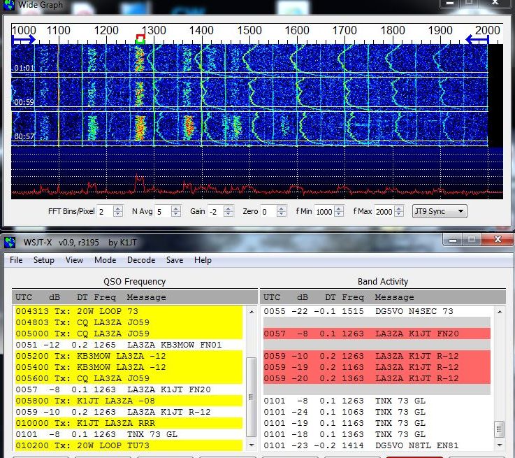Multiple decodes at 100 Hz spacing of K1JT
on 30 m on 28 April 2013, 0101 UTC

From time to time I receive duplicate ‘ghost’ decodes at 100 Hz intervals on either side of the main signal. Last night I saw the phenomenon on 30 m. You will notice here that I have decoded the message: “TNX 73 GL” four times (press image for better readability):

-24 dB, 1063 Hz
-19 dB, 1163 Hz
-8 dB, 1263 Hz
-18 dB, 1363 Hz

The actual contact took place at the frequency of the strongest one, 1263 Hz. The station is only moderately strong at -8 dB and at +/- 100 Hz the first sidebands are 10-11 dB down and at -200 Hz the second one is 16 dB down.

In the post “Ghosts on JT9-1” Julian, G4ILO speculated that it had to do with strong signals. His best example showed a very strong example with signal strength as high as 19 dB and with the +/- 100 Hz ghosts 37-40 dB down, much more than in my example. A commenter proposed that it had to do with the mains frequency and that a North American station should have ghosts at +/-120 Hz instead.

In his second posting, “Ghostly signals“, Julian did some tests and found that a mains power supply can indeed result in weak 100 Hz sidebands. Then it was commented on the wsjtgroup that in the US people see these ghosts at a spacing of 120 Hz and that tests suggest that they are generated at the transmitter end.

But my example is from a US station, and the ghosts are still at +/- 100 Hz, so that theory does not seem to be right. My example indicates that it has to do with the receiver and not the transmitter. It comes and goes and the relative levels seem to vary a lot. My guess is that it is 50/100 Hz that enters the audio signal between the receiver and the PC. The software was the latest v0.9, r3195.

And by the way, the US station in my example happens to be Joe Taylor, K1JT, the originator of the JT9 mode and the decoding software.

Overmodulated JT65 on HF?

April 19th, 2013 |

Author: Sverre LA3ZA

Sometimes it is crowded on JT65 on HF due to too little bandwidth. When only 2 kHz is available and each signal needs 175 Hz that’s understandable. But then others seem to complain that some overmodulate their transmitters so that they occupy more than the 175 Hz, making it even harder to fit an extra signal in the band.

As I have been running a lot of JT65 lately on HF, I also have seen this phenomenon and it pickled my interest to try to understand what was going on. The image below shows such a strong station to the very left, at about -1000 Hz where the red marker is located. After some seconds I turned on the attenuator of my K3, so the signal was attenuated by 10 dB (press image for zoom).

What one can see is that what appears initially (at the bottom of the waterfall) as a splattering signal, becomes quite fine when the attenuator is turned on. Then it spills into neighboring frequencies again as the attenuator is turned off again.

It appears then that it is the JT65 decoder software which is too sensitive to strong signals. Now, I cannot really say that I understand all of the decoder code, but I think that it has to do with the way the power spectrum is estimated. The FORTRAN code for ps.f is listed below. It comes from the BerliOS repository for WSJT which has the same code for this routine as JT65-HF-Comfort:

subroutine ps(dat,nfft,s)

parameter (NMAX=16384+2)

parameter (NHMAX=NMAX/2-1)

real dat(nfft)

real s(NHMAX)

real x(NMAX)

complex c(0:NHMAX)

equivalence (x,c)

nh=nfft/2

do i=1,nfft

x(i)=dat(i)/128.0 !### Why 128 ??

enddo

call xfft(x,nfft)

fac=1.0/nfft

do i=1,nh

s(i)=fac*(real(c(i))**2 + aimag(c(i))**2)

enddo

return

end

What is apparent here is that the raw data, dat, is just put directly into the Fast Fourier Transform routine, xfft, after scaling. There is no windowing function. A window function tapers down the beginning and end of the data set. Window functions in spectral analysis are somewhat involved and I refer to the Wikipedia article for details. But when there is no window function (= rectangular window), the first sidelobe is only 13 dB down from the mainlobe. So that could be why a 10 dB attenuator is enough to remove most of the spillover into adjacent frequencies above.

This could be remedied by using a smooth window function. There are many to chose from, but let’s take a Hamming window as an example, with its first sidelobe 43 dB down. This means that if the data had been multiplied by this taper, the dynamic range would have been in the order of 30 dB higher. But as data is lost by the tapering, the downside is that the bin width increases. For this particular window the noise bandwidth goes up by a factor of 1.36 so sensitivity would suffer by 10log(1.36) or about 1.3 dB (ref: Harris, “On the use of Windows for Harmonic Analysis with the Discrete Fourier Transform,” Proc. IEEE, 1978). There could potentially be other negative side effects on decoding also which I cannot foresee from the limited time I have used in trying to understand the algorithms.

My first impression from using the new JT9 mode is that the problem is much smaller there than for JT65, so maybe something like what I am discussing here has been done in the decoder software. But as far as I know, the source code has not been releasted into the public domain yet by K1JT, so I cannot verify it now.

But it seems clear to me that what looks like splatter has much less to do with overdriving and overmodulating transmitters than one may think, and more to do with the particular way that the spectral estimate is found in the JT65 decoder software. Combined with the variable propagation which is an intrinsic feature of HF and which may create a highly variable signal strength, this is what seems to create the spillover.

Half a year of APRS temperature monitoring

December 28th, 2012 |

Author: Sverre LA3ZA

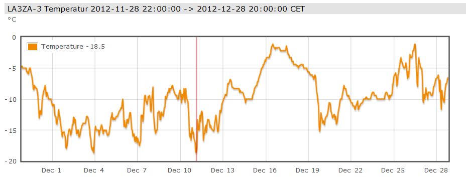My APRS-based temperature monitor has now worked flawlessly for half a year. APRS stands for Automatic Packet Reporting System so it can send much more than temperature data, the chief usage is really for GPS position reports.

But I just needed a temperature monitor and here are the readings for December. As one can see, there were no days with temperature above freezing. At 800 m elevation in the mountains of Telemark in Norway, this is not unexpected for this time of year and makes for good skiing!

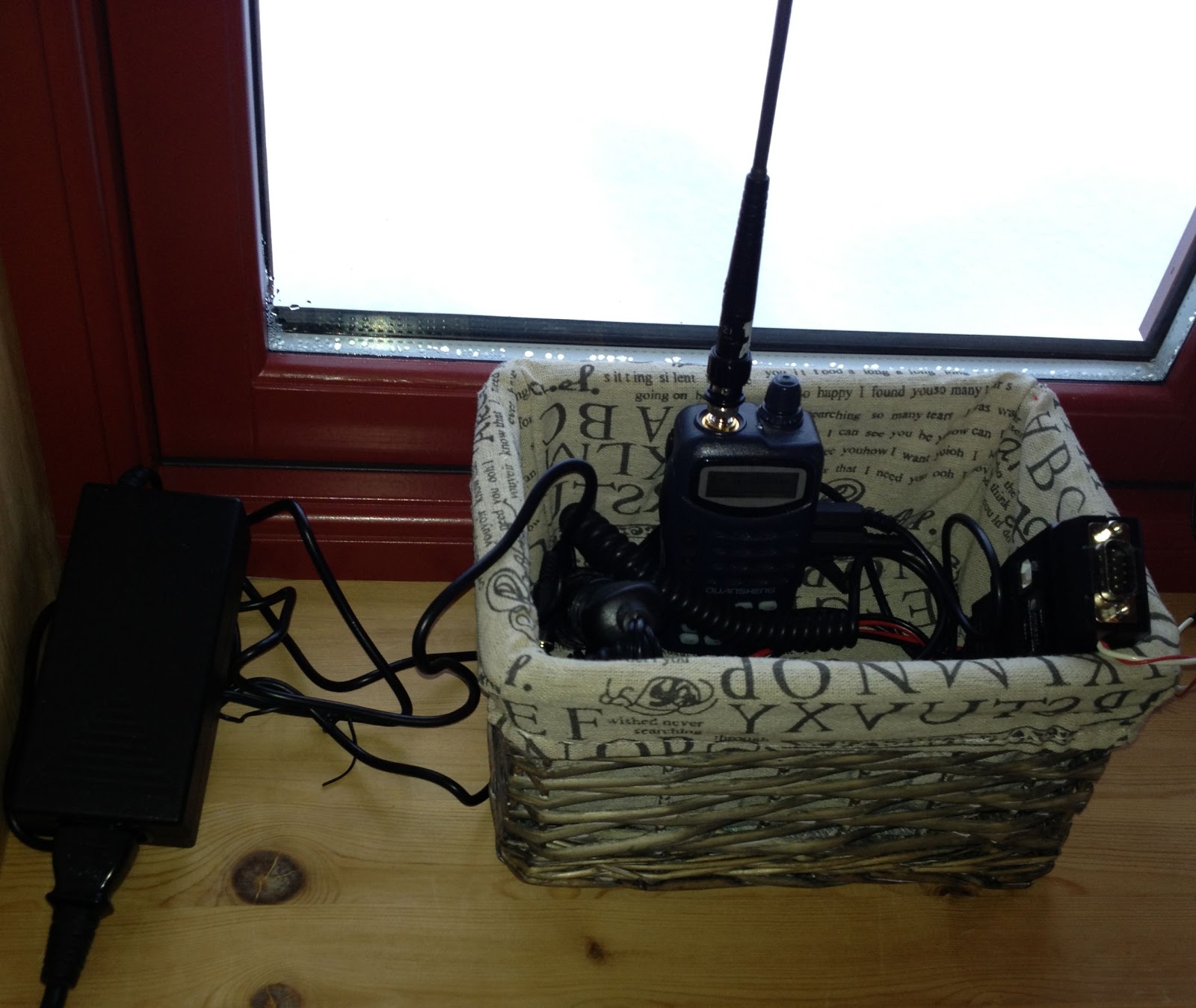
I use a Quanzheng TG-25AT handheld with a quarter-wave whip antenna on 144.800 MHz. Its signals reach the LD3GT digipeater at 1845 m above sea level. Although I don’t have direct line of sight, the low power (1 Watt) setting is adequate as the distance is only 10 km. The APRS-beacon is an OpenTracker USB set up for transmission every 15 minutes. An external DS18S20 temperature sensor which measures the outside temperature is connected to the 1-Wire® bus of the OpenTracker USB.

Thanks to the infrastructure providers: The Tønsberg group of NRRL (LA1T) who operate the LD3GT digipeater, probably the one with the largest coverage in Southern Norway (Gaustadtoppen). Thanks also to the various operators who receive packets from LD3GT and pass them on to the internet, and thanks to aprs.fi for processing and displaying the data on their excellent web site!